Time-Weighting Predictive Models

Why Weight by Time?

In my previous post, I showed how to build a basic Poisson model to predict football match outcomes and explained its main limitation: it treats all historical matches equally, ignoring that teams change over time due to new players, coaches, and evolving tactics.

The Dixon-Coles Weighting Function

In 1997, statisticians Dixon and Coles proposed a solution for this, concluding that recent games are more relevant, and developed a weighting function to reflect this:

Where:

• $t$ is the time elapsed since the game was played
• $\xi$ is a decay parameter. A higher $\xi$ means the weight of older games decreases more rapidly (we care more about newer games).

Dixon and Coles used half-weeks as their time unit and found that $\xi = 0.0065$ gave the best results. They didn’t explain why they chose half-weeks, but probably because it aligns well with the typical schedule of a league (one match per team per week).

Here’s the Python function to calculate weights based on this exponential decay:

import numpy as np

def calculate_weights(dates, xi=0.0065):
    latest_date = dates.max()
    # Difference in days, then convert to half-weeks by dividing by 3.5
    diff_half_weeks = ((latest_date - dates).dt.days) / 3.5
    return np.exp(-xi * diff_half_weeks)

This function takes a series of match dates and returns a weight for each, giving more importance to recent games. We then assign these weights to the model data (model_df from the previous post). And since model_df has two rows per match (home and away), we duplicate each weight accordingly.

And finally, we pass these weights to the fitting function, typically via the freq_weights or weights argument, depending on the GLM implementation.

Is the Original Decay Rate Still Valid?

The Dixon-Coles paper is from 1997, but football has changed a lot since then. Teams now play 50–80 matches per season, players face overloaded schedules, and tactics evolve quickly as teams are data-driven these days. Moreover, your data and model features likely differ from those used by Dixon and Coles. That means you need to find the decay rate to your own dataset and not assume 0.0065 is optimal today.

To visualize how how quickly historical matches lose relevance under various decay rates, here’s a chart showing the decay curves for several values:

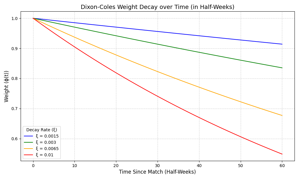
A higher $\xi$ makes older matches matter less, and recent ones count more.

Finding the Best Decay Parameter

The optimal decay parameter is usually found through hyperparameter tuning via cross-validation on training data. You test a range of values (e.g., 0.003, 0.005, 0.0065, 0.008, 0.01, etc.) and pick the one that performs best based on metrics like log-likelihood or Brier score.

Here’s the script:

import pandas as pd
import numpy as np
from scipy.stats import poisson
from sklearn.model_selection import train_test_split
# Read the previous post
from prediction_functions import predict_expected_goals, fit_poisson_model

def calculate_log_likelihood(test_df, model):
    ll_values = []
    for _, row in test_df.iterrows():
        home_xg, away_xg = predict_expected_goals(model, row['home_team'], row['away_team'])
        if all(x > 0 and np.isfinite(x) for x in [home_xg, away_xg]):
            ll = poisson.logpmf(row['home_goals'], home_xg) + poisson.logpmf(row['away_goals'], away_xg)
            if np.isfinite(ll):
                ll_values.append(ll)
    return np.mean(ll_values) if ll_values else np.nan, len(ll_values)

def test_xi_values(xi_values):
    # Load and prepare data
    # Data is from 2015/2016 to 2020/2021
    df = pd.read_csv('data/matches_premier_league.csv')
    df['Date'] = pd.to_datetime(df['Date'])
    # Turn off the shuffling of the data to not mess up the order!
    train_df, test_df = train_test_split(df, random_state=0, shuffle=False)
    
    # Test each xi value
    results = []
    for xi in xi_values:
        weights = calculate_weights(df.Date, xi)
        model = fit_poisson_model(train_df, weights=weights)
        if model:
            avg_ll, valid_count = calculate_log_likelihood(test_df, model)
            print(f"xi={xi:.4f}: Log Likelihood={avg_ll:.4f}, Valid Matches={valid_count}")
            if np.isfinite(avg_ll):
                results.append((xi, avg_ll, valid_count))
    
    # Find best xi and save results
    if results:
        best_xi, best_ll, _ = max(results, key=lambda x: x[1])
        print(f"\nBest xi: {best_xi:.4f} (Log Likelihood={best_ll:.4f})")
        pd.DataFrame(results, columns=['xi', 'log_likelihood', 'valid_matches']).to_csv(
            'time_weighting_evaluation.csv', index=False)
        
        return best_xi
    return None

if __name__ == "__main__":
    test_xi_values(np.arange(0, 0.0205, 0.0005)) # 0 to 0.02 with step 0.0005

For a model trained on English Premier League data from seasons 2010/2011-2020/2021, the best-performing decay parameter turned out to be 0.012, which is much higher than original 0.0065.

Conclusion

1. Implementing time-weighting using the Dixon-Coles decay function makes Poisson models a bit more responsive to current form.
2. The decay rate (0.0065) from original paper may not apply to your data. The best rate depends on your dataset size, and model complexity — you must tune it yourself.
3. Time-weighting is an good improvement, but still only a fraction of what can be done to build a reliable predictive model. There’s always more to explore.